database

Syntax

database(directory, [partitionType], [partitionScheme], [locations], [engine=’OLAP’], [atomic=’TRANS’])

Starting from 1.30.16/2.00.4, if the configuration paramter enableChunkGranularityConfig = true, use the following syntax:

database(directory, [partitionType], [partitionScheme], [locations], [engine=’OLAP’], [atomic=’TRANS’], [chunkGranularity=’TABLE’])

Arguments

directory the directory where a database is located. To establish a database in the distributed file system, directory should start with “dfs://”.

partitionType the partition type could be: sequential (SEQ), range (RANGE), value (VALUE), list (LIST), and composite (COMPO).

partitionScheme the partition scheme describes how the partitions are created. PartitionScheme is usually a vector, with the exception that it is an integer scalar for the sequential domain. The interpretation of the partition scheme depends on the partition type. partitionScheme supports the following data types: CHAR, SHORT, INT, DATE, MONTH, TIME, MINUTE, SECOND, DATETIME, and SYMBOL.

Partition Type	Partition Type Symbol	Partition Scheme
sequential domain	SEQ	An integer scalar. It means the number of partitions.
range domain	RANGE	A vector. Any two adjacent elements of the vector define the range for a partition.
hash domain	HASH	A tuple. The first element is the data type of partitioning column. The second element is the number of partitions.
value domain	VALUE	A vector. Each element of the vector defines a partition.
list domain	LIST	A vector. Each element of the vector defines a partition.
composite domain	COMPO	A vector. Each element of the vector is a database handle.

For a composite database, the vector can contain two or three elements and the length of the vector indicates the partition levels.

locations a tuple indicating the locations of each partition. The number of elements in the tuple should be the same as that of partitions determined by partitionType and partitionScheme. When saving partitions on multiple nodes, we can specify the location for each partition by using the DFS (Distributed File System) or the locations parameter. If the locations parameter is not specified, all partitions reside in the current node. We cannot specify partition locations for composite partitions.

engine = ‘OLAP’ is a parameter with fixed value. Only version 2.00 supports modifying the parameter.

atomic indicates at which level the atomicity is guaranteed for a write transaction, thus determining whether concurrent writes to the same chunk are allowed. It can be ‘TRANS’ or ‘CHUNK’ and the default value is ‘TRANS’.

• ‘TRANS’ indicates that the atomicity is guaranteed at the transaction level. If a transaction attempts to write to multiple chunks and one of the chunks is locked by another transaction, a write-write conflict occurs, and all writes of the transaction fail. Therefore, setting atomic =’TRANS’ means concurrent writes to a chunk are not allowed.

• ‘CHUNK’ indicates that the atomicity is guaranteed at the chunk level. If a transaction tries to write to multiple chunks and a write-write conflict occurs as a chunk is locked by another transaction, instead of aborting the writes, the transaction will keep writing to the non-locked chunks and keep attempting to write to the chunk in conflict until it is still locked after a few minutes. Therefore, setting atomic =’CHUNK’ means concurrent writes to a chunk are allowed. As the atomicity at the transaction level is not guaranteed, the write operation may succeed in some chunks but fail in other chunks. Please also note that the write speed may be impacted by the repeated attempts to write to the chunks that are locked.

chunkGranularity is a string indicating the chunk granularity. It determines whether concurrent writes to different tables in the same chunk are allowed. It is only enabled when enableChunkGranularityConfig = true is configured. The value can be ‘TABLE’ or ‘DATABASE’:

• ‘TABLE’: the chunk granularity is at the TABLE level. In this case, concurrent writes to different tables in the same partition are allowed.

• ‘DATABASE’: the chunk granularity is at the DATABASE level. In this case, concurrent writes to different tables in the same partition are not allowed.

The chunk granularity determines where a DolphinDB transaction locates the lock. Before version 1.30.16/2.00.4, the chunk granularity is at the DATABASE level, i.e., each partition of the database is a chunk. Starting from version 1.30.16/2.00.4, the default chunk granularity is at the TABLE level and each table of the partition is a chunk.

Details

Create a database handle.

To create a new distributed database, we need to specify partitionType and partitionScheme. When we reopen an existing distributed database, we only need to specify directory. We cannot overwrite an existing distributed database with a different partitionType or partitionScheme

Examples

1. To establish a non-partitioned database on disk:

$ db=database(directory="C:/DolphinDB/Data/db1/");
$ t=table(take(1..10,10000000) as id, rand(10,10000000) as x, rand(10.0,10000000) as y);
$ saveTable(db, t, `t1);

2. For distributed database, we give an example for each type of partition:

In a sequential domain (SEQ), the partitions are based on the order of rows in the input data file. It can only be used in the local file system, not in the distributed file system.

$ n=1000000
$ ID=rand(100, n)
$ dates=2017.08.07..2017.08.11
$ date=rand(dates, n)
$ x=rand(10.0, n)
$ t=table(ID, date, x);
$ saveText(t, "C:/DolphinDB/Data/t.txt");

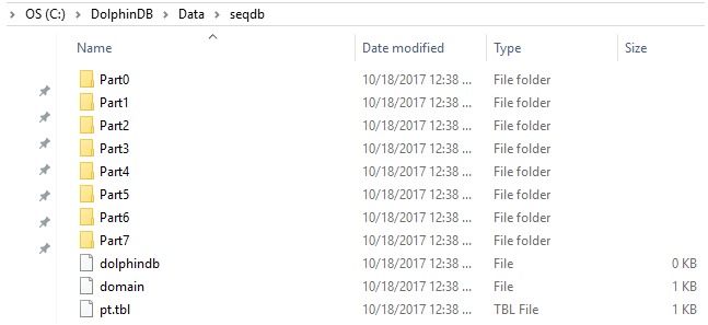
$ db = database(directory="C:/DolphinDB/Data/seqdb", partitionType=SEQ, partitionScheme=8)
$ pt = loadTextEx(db, `pt, ,"C:/DolphinDB/Data/t.txt");

Under the folder “C:/DolphinDB/data/seqdb”, 8 sub folders have been created. Each of them corresponds to a partition of the input data file. If the size of the input data file is larger than the available memory of the computer, we can load the data in partitions.

In a range domain (RANGE), partitions are determined by any two adjacent elements of the partition scheme vector. The starting value is inclusive and the ending value is exclusive.

$ n=1000000
$ ID=rand(10, n)
$ x=rand(1.0, n)
$ t=table(ID, x);
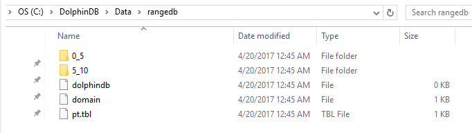
$ db=database(directory="dfs://rangedb", partitionType=RANGE, partitionScheme=0 5 10)
$ pt = db.createPartitionedTable(t, `pt, `ID);
$ pt.append!(t);

$ pt=loadTable(db,`pt)
$ x=select * from pt
$ select count(x) from pt;

count_x
1000000

In the example above, the database db has two partitions: [0,5) and [5,10). Table t is saved as a partitioned table pt with the partitioning column of ID in database db.

To import a data file into a distributed database of range domain in the local file system:

$ n=1000000
$ ID=rand(10, n)
$ x=rand(1.0, n)
$ t=table(ID, x);
$ saveText(t, "C:/DolphinDB/Data/t.txt");

$ db=database(directory="dfs://rangedb", partitionType=RANGE, partitionScheme=0 5 10)
$ pt = loadTextEx(db, `pt, `ID, "C:/DolphinDB/Data/t.txt");

In a hash domain (HASH), the data type and numbers of partitions need to be specified.

$ n=1000000
$ ID=rand(10, n)
$ x=rand(1.0, n)
$ t=table(ID, x)
$ db=database(directory="dfs://hashdb", partitionType=HASH, partitionScheme=[INT, 2])

$ pt = db.createPartitionedTable(t, `pt, `ID)
$ pt.append!(t);

$ select count(x) from pt;

count_x
1000000

In example above, database db has two partitions. Table t is saved as pt(a partitioned table) with the partitioning column ID.

Note: For a database to be imported to a hash domain, if a partitioning column contains NULL value, the record is discarded.

$ ID = NULL 3 6 NULL 9
$ x = rand(1.0, 5)
$ t1 = table(ID, x)
$ pt.append!(t1)
$ select count(x) from pt;

count_x
1000003

In a value domain (VALUE), each element of the partition scheme vector determines a partition.

$ n=1000000
$ month=take(2000.01M..2016.12M, n);
$ x=rand(1.0, n);
$ t=table(month, x);

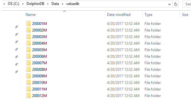
$ db=database(directory="dfs://valuedb", partitionType=VALUE, partitionScheme=2000.01M..2016.12M)
$ pt = db.createPartitionedTable(t, `pt, `month);
$ pt.append!(t);

$ pt=loadTable(db,`pt)
$ select count(x) from pt;

count_x
1000000

The example above defines a database db with 204 partitions. Each of these partitions is a month between January 2000 and December 2016. With function createPartitionedTable and append!, table t is saved as a partitioned table pt in the database db with the partitioning column of month.

In a list domain (LIST), each element of the partition scheme vector determines a partition.

$ n=1000000
$ ticker = rand(`MSFT`GOOG`FB`ORCL`IBM,n);
$ x=rand(1.0, n);
$ t=table(ticker, x);

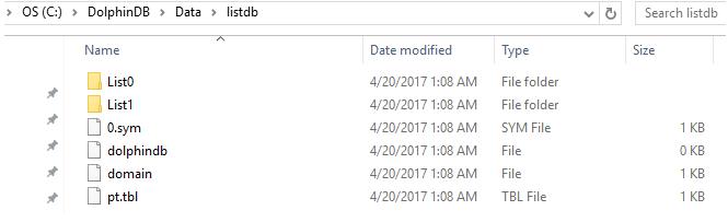
$ db=database(directory="dfs://listdb", partitionType=LIST, partitionScheme=[`IBM`ORCL`MSFT, `GOOG`FB])
$ pt = db.createPartitionedTable(t, `pt, `ticker)
$ pt.append!(t);

$ pt=loadTable(db,`pt)
$ select count(x) from pt;

count_x
1000000

The database above has 2 partitions. The first partition has 3 tickers and the second has 2 tickers.

In a composite domain (COMPO), we can have 2 or 3 partitioning columns. Each column can be of range, value, or list domain.

$ n=1000000
$ ID=rand(100, n)
$ dates=2017.08.07..2017.08.11
$ date=rand(dates, n)
$ x=rand(10.0, n)
$ t=table(ID, date, x)

$ dbDate = database(, partitionType=VALUE, partitionScheme=2017.08.07..2017.08.11)
$ dbID = database(, partitionType=RANGE, partitionScheme=0 50 100)
$ db = database(directory="dfs://compoDB", partitionType=COMPO, partitionScheme=[dbDate, dbID])

$ pt = db.createPartitionedTable(t, `pt, `date`ID)
$ pt.append!(t)

$ pt=loadTable(db,`pt)
$ select count(x) from pt;

count_x
1000000

The value domain has 5 partitions for 5 days:

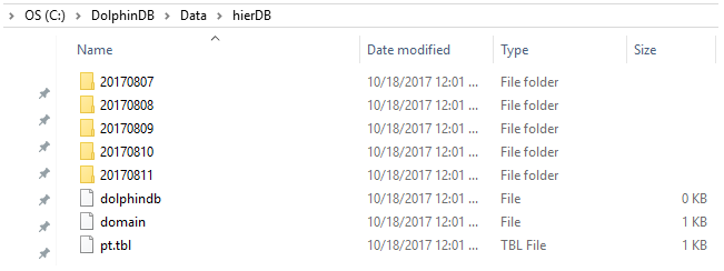
The range domain has 2 partitions:

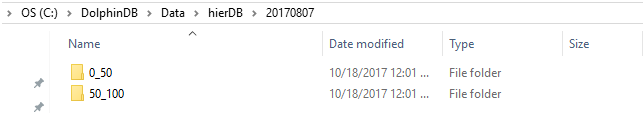
Please note that the although we have 2 levels of folders here for database files, composite domain only has one level of partition. In comparision, there are 2 levels of partition in dual partition.

3. To establish distributed databases in the distributed file system, we can follow the syntax of the examples above. The only difference is that the directory parameter in function database should start with “dfs://”.

To execute the following examples, we need to start a DFS cluster on the web interface, and submit the script on a data node. For details please check “Deployment Guide”.

Save a partitioned table of composite domain in the distributed file system:

$ n=1000000
$ ID=rand(100, n)
$ dates=2017.08.07..2017.08.11
$ date=rand(dates, n)
$ x=rand(10.0, n)
$ t=table(ID, date, x);

$ dbDate = database(, partitionType=VALUE, partitionScheme=2017.08.07..2017.08.11)
$ dbID=database(, partitionType=RANGE, partitionScheme=0 50 100);
$ db = database(directory="dfs://compoDB", partitionType=COMPO, partitionScheme=[dbDate, dbID]);
$ pt = db.createPartitionedTable(t, `pt, `date`ID)
$ pt.append!(t);

The data are stored at a location specified by the configuration parameter volumes.

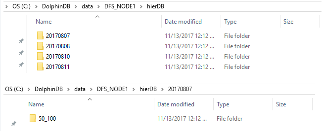
Please note that DFS_NODE1 only has 4 date folders; under DFS_NODE1, the folder of 20170807 only has 1 ID folder. This is because here we have 4 data nodes and 2*5=10 partitions based on date and ID. By default each partition has 3 copies in the distributed file system. Therefore, we have 5*2*3=30 partitions in total saved on 4 data nodes. Not all data nodes have all the 10 partitions.

Import a data file into a distributed database of range domain in the distributed file system:

$ n=1000000
$ ID=rand(10, n)
$ x=rand(1.0, n)
$ t=table(ID, x);
$ saveText(t, "C:/DolphinDB/Data/t.txt");

$ db=database("dfs://rangedb", RANGE,  0 5 10)
$ pt = loadTextEx(db, `pt, `ID, "C:/DolphinDB/Data/t.txt");

4. Examples regarding the locations parameter:

$ n=1000000
$ ID=rand(10, n)
$ x=rand(1.0, n)
$ t=table(ID, x);

$ db=database(directory="dfs://rangedb5", partitionType=RANGE, partitionScheme=0 5 10, locations=[`node1`node2, `node3])
$ pt = db.createPartitionedTable(t, `pt, `ID);
$ pt.append!(t);

The example above defines a list domain that has 2 partitions. The first partition resides on 2 sites: node1 and node2, and the second partition resides on site node3. All referred sites must be defined in the sites attribute of dolphindb.cfg on all machines where these nodes are located:

$ sites=111.222.3.4:8080:node1, 111.222.3.5:8080:node2, 111.222.3.6:8080:node3

Sites are separated by comma. Each site specification contains 3 parts: host name, port number, and alias. A partition can reside on multiple sites that back up each other. In this example, each node is located on a different machine.

We can also use the actual host name and the port number to represent a site. The function call can be changed to

$ db=database("C:/DolphinDB/Data/rangedb6", RANGE, 0 5 10, [["111.222.3.4:8080", "111.222.3.5:8080"], "111.222.3.6:8080"])

5. Examples regarding the parameter atomic:

$ if(existsDatabase("dfs://test"))
$ dropDB("dfs://test")
$ db = database(directory="dfs://test", partitionType=VALUE, partitionScheme=1..20, atomic='CHUNK')
$ dummy = table(take(1..20, 100000) as id, rand(1.0, 100000) as value)
$ pt = db.createPartitionedTable(dummy, "pt", `id)

$ dummy1 = table(take(1..15, 1000000) as id, rand(1.0, 1000000) as value)
$ dummy2 = table(take(11..20, 1000000) as id, rand(1.0, 1000000) as value)
$ submitJob("write1", "writer1", append!{pt, dummy1})
$ submitJob("write2", "writer2", append!{pt, dummy2})
$ submitJob("write3", "writer3", append!{pt, dummy1})
$ submitJob("write4", "writer4", append!{pt, dummy2})
$ select count(*) from pt
4,000,000